A hidden Markov model (HMM) is a statistical Markov model in which the system being modeled is assumed to be a Markov process with unobserved (hidden) states. An HMM can be considered as the simplest dynamic Bayesian network.
In a regular Markov model, the state is directly visible to the observer, and therefore the state transition probabilities are the only parameters. In a hidden Markov model, the state is not directly visible, but output, dependent on the state, is visible. Each state has a probability distribution over the possible output tokens. Therefore the sequence of tokens generated by an HMM gives some information about the sequence of states. Note that the adjective 'hidden' refers to the state sequence through which the model passes, not to the parameters of the model; even if the model parameters are known exactly, the model is still 'hidden'.
Hidden Markov models are especially known for their application in temporal pattern recognition such as speech, handwriting, gesture recognition, part-of-speech tagging, musical score following, partial discharges and bioinformatics.
A hidden Markov model can be considered a generalization of a mixture model where the hidden variables (or latent variables), which control the mixture component to be selected for each observation, are related through a Markov process rather than independent of each other.
2. Key Points:
1. Set of states:
2. Process moves from one state to another generating a sequence of states :
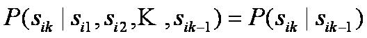
3. Markov chain property: probability of each subsequent state depends only on what was the previous state:
4. States are not visible, but each state randomly generates one of M observations (or visible states)
5. To define hidden Markov model, the following probabilities have to be specified: matrix of transition probabilities A=(aij), aij= P(si | sj) , matrix of observation probabilities B=(bi (vm )), bi(vm ) = P(vm | si ) and a vector of initial probabilities p=(pi), pi = P(si) . Model is represented by M=(A, B, p).
3. Example of Hidden Markov Model:
$IMAGE5$
1. Two states : ‘Low’ and ‘High’ atmospheric pressure.
2. Two observations : ‘Rain’ and ‘Dry’.
3. Transition probabilities: P(‘Low’|‘Low’)=0.3 , P(‘High’|‘Low’)=0.7 , P(‘Low’|‘High’)=0.2, P(‘High’|‘High’)=0.8
4. Observation probabilities : P(‘Rain’|‘Low’)=0.6 , P(‘Dry’|‘Low’)=0.4 , P(‘Rain’|‘High’)=0.4 , P(‘Dry’|‘High’)=0.3
5. Initial probabilities: say P(‘Low’)=0.4 , P(‘High’)=0.6
4. Calculation of observation sequence probability
1. Suppose we want to calculate a probability of a sequence of observations in our example, {‘Dry’,’Rain’}.
2. Consider all possible hidden state sequences:
P({‘Dry’,’Rain’} ) = P({‘Dry’,’Rain’} , {‘Low’,’Low’}) + P({‘Dry’,’Rain’} , {‘Low’,’High’}) + P({‘Dry’,’Rain’} , {‘High’,’Low’}) + P({‘Dry’,’Rain’} , {‘High’,’High’})
where first term is :
P({‘Dry’,’Rain’} , {‘Low’,’Low’})= P({‘Dry’,’Rain’} | {‘Low’,’Low’}) P({‘Low’,’Low’}) = P(‘Dry’|’Low’)P(‘Rain’|’Low’) P(‘Low’)P(‘Low’|’Low) = 0.4*0.4*0.6*0.4*0.3
where first term is :
P({‘Dry’,’Rain’} , {‘Low’,’Low’})= P({‘Dry’,’Rain’} | {‘Low’,’Low’}) P({‘Low’,’Low’}) = P(‘Dry’|’Low’)P(‘Rain’|’Low’) P(‘Low’)P(‘Low’|’Low) = 0.4*0.4*0.6*0.4*0.3
5. Main issues using HMMs:
1. Evaluation problem: Given the HMM M=(A, B, p) and the observation sequence O=o1 o2 ... ok, calculate the probability that model M has generated sequence O .
2. Decoding problem: Given the HMM M=(A, B, p) and the observation sequence O=o1 o2 ... ok, calculate the most likely sequence of hidden states sithat produced this observation sequence O.
3. Learning problem: Given some training observation sequences O=o1 o2 ... ok and general structure of HMM (numbers of hidden and visible states), determine HMM parameters M=(A, B, p) that best fit training data.
O=o1 o2 ... ok denotes a sequence of observations ok€{v1,…,vM}.