| Section categories |
|
Related Subjects [38]
This category includes brief overview of all related subjects.
|
|
Defining BioInformatics [7]
In this section we tried to briefly explain what bioinformatics is ?
|
|
Unviersities [30]
This contains information about universities that are offering bioinformatics degree programs.
|
|
Resources [24]
Contains information about bioinformatics resources including databases, tools and techniques.
|
|
Algorithms [31]
This category includes some of the basic algorithms that are usually used by bioinformaticians.
|
|
| Statistics |
Total online: 1 Guests: 1 Users: 0 |
|
Home » 2011 » August » 23 » Neighbor Joining
|
Neighbor Joining
1. Description: In bioinformatics, neighbor joining is a bottom-up clustering method for the creation of phenetic trees (phenograms), created by Naruya Saitou and Masatoshi Nei. Usually used for trees based on DNA or protein sequence data, the algorithm requires knowledge of the distance between each pair of taxa (e.g., species or sequences) to form the tree.
2. Key Points: - Most widely-used distance based method for phylogenetic reconstruction
- UPGMA illustrated that it is not enough tojust pick closest neighbors
- Idea here: take into account averageddistances to other leaves as well
- Produces an unrooted tree
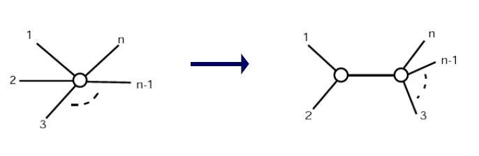
Start off with star tree; pull out pairs at a time
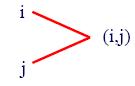
3. NJ Algorithm: - Step 1: Let
 - (Almost) "average” distance to other nodes
- Step 2: Choose i and j for which Mij – ui –uj is smallest
- Look for nodes that are close to each other,and far from everything else
- Turns out minimizing this is minimizing sum of branch lengths
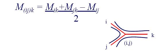
- Step 3: Define a new cluster (i, j), with a corresponding node in the tree
 - Distance from i and j to node (i,j):
- di, (i,j) = 0.5(Mij + ui-uj)
- dj, (i,j) = 0.5(Mij +uj-ui)
- Default: split distance but if on average one is further away, make it longer
- Step 4: Compute distance between new cluster and all other clusters:
- Step 5: Delete i and j from matrix and replace by (i, j)
- Step 6: Continue until only 2 leaves remain
4. Example: Let us assume that we have four taxa (A, B, C, D) and the following distance matrix: | A | B | C | D |
|---|
| A | 0 | 7 | 11 | 14 |
|---|
| B | 7 | 0 | 6 | 9 |
|---|
| C | 11 | 6 | 0 | 7 |
|---|
| D | 14 | 9 | 7 | 0 |
|---|
We obtain the following values for the Q matrix: | A | B | C | D |
|---|
| A | 0 | −40 | −34 | −34 |
|---|
| B | −40 | 0 | −34 | −34 |
|---|
| C | −34 | −34 | 0 | −40 |
|---|
| D | −34 | −34 | −40 | 0 |
|---|
In the example above, two pairs of taxa have the lowest value, namely −40. We can select either of them for the second step of the algorithm. We follow the example assuming that we joined taxa A and B together. If u denotes the new node, then the branch lengths of edges {A,u}and {B,u} are respectively 6 and 1, by the above formula. We then proceed to updating the distance matrix, by computing d(u,k) according to the above formula for every node k. In this case, we obtain d(u,C) = 5 and d(u,D) = 8. The resulting distance matrix is: We can start the procedure anew taking this matrix as the original distance matrix. In our example, it suffices to do one more step of the recursion to obtain the complete tree. 5. Advantages And Disadvantages: Neighbor joining is based on the minimum-evolution criterion, i.e. the topology that gives the least total branch length is preferred at each step of the algorithm. However, neighbor joining may not find the true tree topology with least total branch length because it is a greedy algorithm that constructs the tree in a step-wise fashion. Even though it is sub-optimal in this sense, it has been extensively tested and usually finds a tree that is quite close to the optimal tree. Nevertheless, it has been largely superseded by phylogenetic methods that do not rely on distance measures and offer superior accuracy under most conditions. The main virtue of neighbor joining relative to these other methods is its computational efficiency. That is, neighbor joining is a polynomial-time algorithm. It can be used on very large data sets for which other means of analysis (e.g. minimum evolution, maximum parsimony, maximum likelihood) are computationally prohibitive. Unlike the UPGMA algorithm for tree reconstruction, neighbor joining does not assume that all lineages evolve at the same rate (molecular clock hypothesis) and produces an unrooted tree. Rooted trees can be created by using an outgroup and the root can then effectively be placed on the point in the tree where the edge from the outgroup connects. Furthermore, neighbor joining is statistically consistent under many models of evolution. Hence, given data of sufficient length, neighbor joining will reconstruct the true tree with high probability. Atteson proved that if each entry in the distance matrix differs from the true distance by less than half of the shortest branch length in the tree, then neighbor joining will construct the correct tree. RapidNJ and NINJA are fast implementations of the neighbor joining algorithm. Although neighbor joining relies on a matrix whose entries are natural, some branch lengths in the resulting topology may be real numbers
6. NJ Performance: - Works well in practice
- If there is a tree that fits the matrix, it will find it
- Can sometimes get trees with negative length edges (!)
|
|
|
Category: Algorithms |
Views: 3513 |
Added by: Ansari
| Rating: 1.0/1 |
|
|
|