Baum–Welch Algorithm
1. Description: In electrical engineering, computer science, statistical computing and bioinformatics, the Baum–Welch algorithm is used to find the unknown parameters of a hidden Markov model (HMM). It makes use of the forward-backward algorithm and is named for Leonard E. Baum and Lloyd R. Welch.
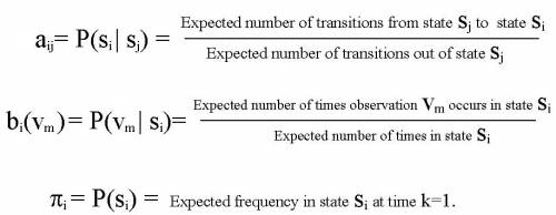
2. Explanation: The Baum–Welch algorithm is a particular case of a generalized expectation- maximization (GEM) algorithm. It can compute maximum likelihood estimates and posterior mode estimates for the parameters (transition and emission probabilities) of an HMM, when given only emissions as training data. For a given cell Si in the transition matrix, all paths to that cell are summed. There is a link (transition from that cell to a cell Sj). The joint probability of Si, the link, and Sj can be calculated and normalized by the probability of the entire string. Call this χ. Now, calculate the probability of all paths with all links emanating from Si. Normalize this by the probability of the entire string. Call this σ. Now divide χ by σ. This is dividing the expected transition from Si to Sj by the expected transitions from Si. As the corpus grows, and particular transitions are reinforced, they will increase in value, reaching a local maximum. No way to ascertain a global maximum is known. 3. General Idea:  4. Expectation Step: Define variable xk(i,j) as the probability of being in state si at time k and in state sj at time k+1, given the observation sequence o1 o2 ... oK.
xk(i,j)= P(qk= si , qk+1= sj | o1 o2 ... oK) Define variable gk(i) as the probability of being in state si at time k, given the observation sequence o1 o2 ... oK. gk(i)= P(qk= si | o1 o2 ... oK) 1. We calculated P(qk= si , qk+1= sj | o1 o2 ... oK) and gk(i)= P(qk= si | o1 o2 ... oK). 2. Expected number of transitions from state si to state sj = Sk xk(i,j) 3. Expected number of transitions out of state si = Sk gk(i) 4. Expected number of times observation vm occurs in state si = Sk gk(i) , k is such that ok= vm
5. Expected frequency in state si at time k=1 : g1(i).
5. Maximization Step:
|


